Section 4 - A Simple Gantt Chart

Manufacturing Corner on

Saturday, November 26, 2022

 The start and stop times of each job are calculated by formulas that cascade down the columns, but as a visual aid, the 

information may also be displayed as a Gantt chart. This is how you set it up:

- to the right of the schedule make narrow columns and head them from hours 1 to 36

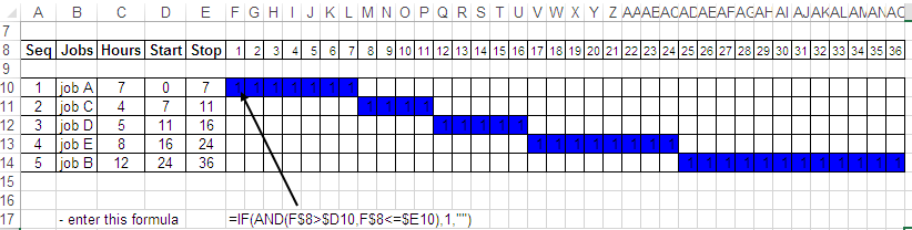
- enter this formula =IF(AND(F$8>$D10,F$8<=$E10),1,"")

  It tests the cell to see whether the hour number in the column heading is between the start 

  and stop.

  If it is, it returns a 1, if not it returns "" (a blank)

 The $'s ensure that when the formula is copied it continues to reference columns D and E for  the start and stop,and row 8 for the hour number.

- set Format|Conditional Formatting|Pattern|Colour if the cell value =1, to emphasize the  

  cell with a colour

- copy the formula in F10, and paste it to the range F10:AO14

    Try changing the figures in the Hours column to see how the Gantt chart responds, or change one of the sequence numbers and sort to re-sequence the schedule.

Labels: Scheduling Excel Basic

Thanks for reading Section 4 - A Simple Gantt Chart. Please share...!